Updated on March 25, 2023
We are not rational when we make choices under risk and uncertainty.
This is because we prefer certainty. We do not want to live in uncertainty.
Look at the following scenarios;
The following examples appear in
Daniel Kahneman and Amos Tversky’s 1979 paper on prospect theory.
Their data were from the responses to hypothetical scenarios presented to Israeli university students.
Scenario 1:
Certainty effect with a monetary outcome gain
Consider that you are given the following two options;
Option A:
A guaranteed win of 2500 in cash.
Option B:
33% chance of winning 2500 in cash or 66% chance of winning 2400.
Which one do you choose?
Option A?
/ That was the option that 82 per cent of Israeli students chose.
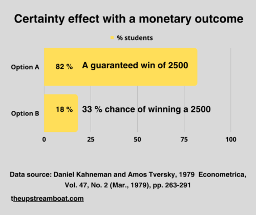
Option A: A guaranteed win of 2500 Israeli pounds
Option B: 33% chance of winning 2500 Israeli pounds or 66% chance of winning 2400.
Now, go to the second scenario.
Scenario 2:
Certainty effect with a non-monetary outcome gain
You are given the following options;
Option 1:
A guaranteed one-week tour of England
Option 2:
50% chance of winning a three-week tour of England, France, and Italy
What are your options?
Again, 78 per cent of students chose the surest option.
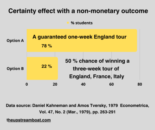
Option A: A guaranteed one-week tour of England
Option B: 50% chance of winning a three-week tour of England, France, Italy
We risk averse for sure gains.
What will we do when we face uncertainty in gains?
Scenario 3:
Uncertainty effect with a non-monetary outcome
Now, consider the following options; in this situation, both options carry minimal chances of winning and the difference between the chances becomes smaller.
Option A:
5 per cent chance to win a three-week tour of England, France, and Italy
Option B:
10 per cent chance to win a one-week tour of England.
Look at what happened; the above choices became reversed.

Option A: 5% chance to win a three-week tour of England, France, Italy
Option B: 10% chance to win a one-week tour of England
In other words, when both options become uncertain and the difference in the uncertainty is smaller, we take the more significant risk for a bigger gain.
However, if the chance differences become substantial, we go for the safer option.
When we face losses;
Scenario 4:
Uncertainty effect with a monetary outcome:
What will we do when one prospect is a sure loss and the other is an almost certain loss?
Now, consider the following gambling options;
Option A:
A sure loss of 3000.
Option B:
80% chance of losing 4000.
Here, the students chose the riskier option in front of a sure loss.
So, students shifted from risk aversion mode to risk seeking mode for gains even with a high probability for a higher amount in spite of sure loss of a smaller amount.
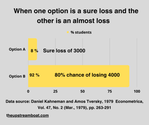
Option A: A sure loss of 3000
Option B: 80% chance of losing 4000
Scenario 5:
When both losses become probable losses
Now, consider when both losses carry different degrees of probability but the difference between the chances becomes substantial.
Option A:
90% chance of losing 3000.
Option B:
45% chance of losing 6000.
Here too, students traded the larger loss with a lower probability over the smaller loss with a higher probability. This is an attempt at risk aversion for losses of lower probability.
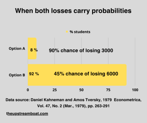
Option A: 90% chance of losing 3000
Option B: 45% chance of losing 6000
Look at the following table and the graph.
What do you notice here?
| First column | Second column | Third column |
| The gamble | You will gain | You will lose |
| 3000 for sure | 80% opted | only 8% opted |
| 4000 for an 80% chance | Only 20% opted | 92% opted |
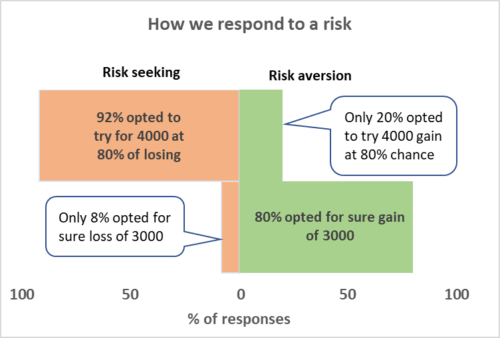
We can notice that when the students chose the surest option of smaller gain, which is 3000 over the risky larger gain, which is 4000 at 80 per cent probability.
On the other hand, students chose the larger but riskier option to avoid the certain loss of the smaller option.
Kahneman and Tversky argue that the certainty effect contributes to both decisions.
When it comes to gains or losses, we think about it in relative terms than absolute terms. This is because our decisions revolve around our perceived reference point (line).
The reference point (line)
How do we determine the gains and losses?
We first draw a reference line.
How?
Think of the following two situations;
Think of the following two situations;
Scenario I:
” you have three bows: the middle one with water at room temperature, the left one with warm water and the right one with cold water;
Now, immerse your left hand in the warm water and the right hand in cold water;
Then, immerse both hands into the middle bowl;
You will experience warmth in the right hand and coldness in the left hand”.
Here, our decision of whether the water is warm or cold varies with the warmth of the water in the middle bowl.
That is the reference point.
Scenario 2:
“Now, think of a situation that turns on a weak light in a dark room and turns on the same light in a brightly lighted room.
You see the difference. t
The weak light has a more significant impact in the dark room.
In our daily lives, most of the time, the reference point is the values and assets at hand at this very moment;
Everything we perceive is relative to the reference line we draw. For example, a certain level of wealth may be considered as abject poverty by one and rich by another. (However, we can change the reference point at any time. It can also be any future standard that we anticipate achieving.)
We call it the “status quo”. This reference point (line) can include,
- Money,
- Any other assets,
- Health,
- Education,
- or any other thing that we own.
This is the first phase of your decision-making process; Khenaman and Tversky call it as the “editing phase”. At first, we create a reference point (line) relative to your present status or expected status. This is where the “framing effect” operates.
Then, we group the available options either as a gain or a loss.
Then, we move on to the second, decision-making phase; which we also call the “evaluation phase”.
Variation of the perceived value for different amounts
Khenaman and Tversky present another interesting phenomenon. Our perceived values are higher for smaller changes than for larger changes.
S-shaped curve:
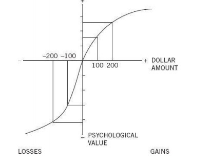
Consider this example;
Think that you increased the amount you had from 100 to 200. and then, think that you increased this amount from 1100 to 1200.
The perceived psychological value of your initial gain tends to be much higher than the perceived value of the latter gain.
The same holds true when we lose money as well. Of course, this applies only if we can tolerate the larger loss.
Khenaman and Tversky showed that the relation between gains and losses and the psychological value we assign to it takes an S-shaped curve as follows;
but, there is a difference. The loss curve is steeper than the gain curve.
What does that mean?
We overweight (overvalue) losses over similar gains.
Losses hurt more than gains gratify.
Jack S. Levy, 1996, p. 181
Jack Levy puts it more simply as follows;
The pleaseure we get from unexpected gain of $10 is much less than the pain we suffer from losing $10.
Jack Levy, 1996
Loss aversion
Because of that, we try our best to prevent losses much more than trying to gain a similar amount; Kahneman and Tversky name it “loss aversion”.
An excellent recent example of loss aversion was stockpiling supplies during the pandemic. At that time, our future reference line was the availability (or scarcity) of essential goods for a living. Assuming there would be a scarcity, we stockpiled to avoid losses.
Endowment effect
Because of our loss aversion, we overvalue what we have at hand. Richard Thaler names it the “endowment effect”. In other words, we get more upset when we lose something than what we were unable to gain.
The endowment effect is much stronger for the physical possession of goods than its virtual counterparts. For example, we do not feel much about spending with credit cards than using coins or paper money.
Diminished sensitivity to loss aversion with time
Much later, in 1992, Tversky and Kahneman updated their original theory as “accumulated prospect theory”. Here, they said that our loss aversion values would diminish with time when similar events accumulate. Researchers use these findings to explain our waning conformity with COVID-19 preventive actions as the pandemic spread with time.
Applications of the Prospect Theory:
- When framing messages:
- We can use the framing effect of the prospect theory to craft our messages both in clinical care and public health. You can find a detailed discussion in this post on how to use the prospect theory to frame messages.
- Prospect theory in conflict resolution:
- Jack Levy discusses the application of the prospect theory in conflict resolution with solid examples. Very much similar to the loss aversion and the endowment effect, he discusses concession aversion between two warring factions on the bargaining table. Both groups may put more weight on concessions rather than what they get in return. This situation may lead to a stalemate. The danger here is that if one faction perceives the concession as a certain or near-certain loss, they might resort to taking very high risky actions to prevent the perceived loss.
- In the finance sector: Banks are more likely to take risks if they perceive that they are running at a loss.
- In the insurance sector: Purchasing an insurance plan is a common example of the prospect theory at work.
- In the consumer choice: We can find many examples of the prospect theory in making choices of buying goods.